PostgreSQL B-Tree Index Explained - PART 1
One can imagine searching a certain explanation in a textbook. One way for this is to read the entire book again. Of course this works, but it will take many hours or even days. Another way is to look in the table of content and to pinpoint based on titles and subtitles the page where the explanation can be found.
The technical purpose of the database index is to limit as much as possible disk IO while executing a query. Therefore if a query retrieves the entire data, there is no point for the database to use an auxiliary structure such as an index because the end result will be reading the entire data from the disk anyway. An index is a separate data structure managed by the database, which be can used while executing a query, in order to avoid reading the entire data for a query that only requires a small part of it.
Different implementations of an index will improve query performance for different type of operators. PostgreSQL comes with many implementations by default for the index data structure[1]:
- B-Tree Index - very useful for single value search or to scan a range, but also for pattern matching.
- Hash Index - very efficient when querying for equality.
- Generalized Inverted Index (GIN) - useful for indexing array values and testing the presence of an item.
- Generalized Search Tree (GiST) - a more complex index structure useful for more exotic searches such as nearest-neighbor or pattern matching.
- Space Partitioned GiST (SP-GiST) - similar with GiST, this index implementation supports space partitioned trees such as quadtrees, k-d trees, and radix trees.
- Block Range Index (BRIN) - this type of index stores summary information for each table block range[2].
Additional to these index types, PostgreSQL comes with an extension to define custom index types [3].
B-Tree indexes are the default option when creating an index without specifying the type. They are very flexible when it comes to operators and data types, which makes them a good choice for a large number of applications. This two part article will focus on a deeper understanding of the inner mechanics of the B-Tree index. The first part of the article will focus on the index data structure and how PostgreSQL uses this structure when executing simple queries, while the second part looks at more complex queries, such as joins and aggregates, and how indexes can influence their performance.
To explain better the mechanics behind the index structure, I will use a PostgreSQL 10 database with two tables: employees and addresses. These two tables will serve as examples for all the code to follow.
CREATE TABLE "public"."addresses" (
    "id" integer NOT NULL,
    "city" character varying(40) NOT NULL,
    "country" character varying(40) NOT NULL,
    "street" character varying(40) NOT NULL
);

CREATE TABLE "public"."employees" (
    "id" integer NOT NULL,
    "company_id" integer NOT NULL,
    "dep" integer NOT NULL,
    "first_name" character varying(20),
    "last_name" character varying(20),
    "salary" integer,
    "address_id" integer
);
In order to create and populate the tables, one can use the script from postgres-btree-dataset and run it inside PostgreSQL CLI:
\i database.sql
B-Tree index structure
As mentioned before, the sole purpose of an index structure is to limit the disk IO while retrieving a small part of data. While searching the disk is a linear operation, the index has do better than linear in order to be useful.
As reflected by the name, the PostgreSQL B-Tree index is based on the B-Tree data structure. To be more precise PostgreSQL B-Tree implementation is based on Lehman & Yao Algorithm[4] and B+-Trees[5].
The difference between B-Trees and B+-Trees is the way keys are stored. In case of B-Tree each key is stored once, either in a non-leaf node or in a leaf node. In case of B+-Trees all keys are present in the leaf nodes and the non-leaf nodes contain duplicates[6]. Fig. 1 illustrates a simplified version a B-Tree Index, which will be used to explain the inner mechanics of PostgreSQL B-Tree index.

Fig.1 Simplified B-tree Index
As one can see in Fig. 1, the linked list from the bottom of the tree stores in each entry access information for multiple table rows: it stores the actual index value, known as key, and also the ROWID which references the table row on the disk. The key is used to locate the table row inside the index structure, while the ROWID is used to locate the table row outside the index. The list items are called leaf nodes.
Above the linked list, the first level of the tree begins. The balanced search tree stores in each of its entries keys and child pointers. In order to access certain ROWIDs from the leaf nodes, this tree is traversed starting from the root until the leaf node, choosing the path by comparing keys on the way. Each tree node is called a non-leaf node or internal node.
Leaf nodes
Level 0 of the index structure is a linked list, which allows traversing all index keys linearly. Each element from a leaf node stores a key and a ROWID. The ROWID points to the corresponding table row outside the index structure.
Between each leaf node elements and between each leaf nodes, there is a logical order based on the index key. This ordering is independent of physical ordering. Because of this independence, operations such as inserts are done very fast due to the fact that it depends only on updating a few pointers without moving around large amounts of data[7]. The linked list also allows the traversal of leaf nodes in the logical order. Finally, PostgreSQL implementation of B-Tree allows the index to be traversed in both ascending and descending order.
Internal nodes
Different from leaf nodes, internal nodes store N keys and also N+1 pointers to siblings instead of ROWID. The keys stored are in ascending order and based on this the pointers help descent into the tree accordingly. If one takes for example the root node from Fig.1, it can see there are two keys and three pointers. In order to find a certain key, each node key is visited from left to right, in ascending order, as long as there are unvisited keys and the searched key is greater than the node key.
With its logarithmic structure, the tree can store millions of keys in just a few levels[7]. Adding more data will have a small impact on the tree traversal. Opposed to the linear search aforementioned, searching for any key is done in logarithmic time[8].
Index lookup
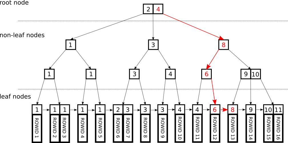
Fig.2 Index lookup
Most of the query performance behaviour is explained by the internal and leaf nodes traversal. These two are the first steps of the index lookup.
As described in SQL Performance Explained[7], an index lookup requires three steps: a tree traversal until the leaf nodes, following the leaf node chain until all matching records are found and fetching the actual data from the disk. Because the tree traversal is limited by the depths of the tree, only the last two steps can strongly influence query performance.
Fig. 2 explains very well the lookup process for key 8. Because 8 is greater than all root keys, the lookup will descent using the last pointer. The first internal node key is equal to the searched key and the lookup will descend using the first pointer. The second internal node key is less than 8, the lookup will descend using the last pointer and reach the leaf node linked list. The lookup will follow the linked list until a value greater than 8 is reached.
Index classification
PostgreSQL indexes have been categorized so far based on their internal implementation, yet they can be also classified based on their utility:
- Single-column index - an index defined on a single table column
- Multi-column index - an index defined on multiple table columns
- Partial index - an index defined on both columns and rows
- Unique index - an index which enforces that the keys in the tree are unique
1. Single-column index
Fig. 1 represents an image of a single column index. Each key represents a single value. In order to see this in practice one can run the simple query that retrieves employees based on their id, such as the one below. Because there is no index yet on the id column of the employees table when running the query, the output does not include any trace of using an index. After creating a primary key on id column (which is an index with a unique constraint), the outcome is different.
Query Example 1
EXPLAIN ANALYZE SELECT first_name FROM employees WHERE id > 1000 AND id < 10000;
                                                 QUERY PLAN
-------------------------------------------------------------------------------------------------------------
 Seq Scan on employees  (cost=0.00..2336.00 rows=9095 width=8) (actual time=0.323..11.812 rows=8999 loops=1)
   Filter: ((id > 1000) AND (id < 10000))
   Rows Removed by Filter: 91001
 Planning time: 0.117 ms
 Execution time: 12.664 ms
(5 rows)
As a short explanation, when executing a query with EXPLAIN, the output is a query plan that describes the steps the database will take in order to deliver the records. More about the PostgreSQL query plan will be covered in the next sections.
In the query plan above, one can see that the database will perform a sequential scan(one can think of sequential scan as reading data from the disk) and will use a filter to eliminate records which do not respect the WHERE condition. Finally it estimates the execution time.
In this plan there is no sign of any index. But to be fair there is no index yet. For the next query, a primary key is added and finally the same query is ran again.
For better exemplification, after each statement that alters a table, a VACUUM ANALYZE is performed in order to refresh database statistics.
Query Example 2
ALTER TABLE employees ADD PRIMARY KEY (id);

VACUUM ANALYZE employees;

EXPLAIN ANALYZE SELECT first_name FROM employees WHERE id > 1000 AND id < 10000;
                                                            QUERY PLAN
----------------------------------------------------------------------------------------------------------------------------------
 Index Scan using employees_pkey on employees  (cost=0.29..343.45 rows=8608 width=8) (actual time=0.043..4.873 rows=8999 loops=1)
   Index Cond: ((id > 1000) AND (id < 10000))
 Planning time: 0.162 ms
 Execution time: 5.771 ms
(4 rows)
The terminology used below will be covered in the next sections. What is important to notice in this example is that the scan and condition type changes once an index can be used. The difference between the two query plans is as follow:
- Index Scan is used instead of Sequential Scan because the database can take advantage of the primary key
- The Filter section was replaced with Index Cond which represents the index lookup condition
- The estimated time is less than the previous run.
2. Multi-column Index

Fig.3 Simplified B-tree Multi-column Index
Along single-column indexes, PostgreSQL supports multi-column indexes up to 32 columns. The key is not represented by a single value, instead it is represented as a tuple. Because the key is not a single value, the index logical order will take into account each value from the tuple. Thus, the index will be ordered by the first key element, then by second key element and so on.
One first good approach when defining multi-column indexes is to find which columns have a smaller granularity within the existing data, and to use them as leading elements in the index definition. For example, in practice, a column that represents an event time will have a bigger granularity than a column that represents a name. In other words, a column that can group the data in fewer groups, but larger in size than any other column, should lead in the index definition. If this is respected for all index columns, then inside each of these large groups, elements will represent a contiguous sorted range within the leaf node chain, thus it will be faster for an index lookup to traverse the leaf nodes once it has found where to start and where to stop, because it can traverse it in one iteration without interruption.
In the current database, the multi-column index will be built using the company, the department and the employee’s last name, in this order. This index reflects a “belonging” relationship: an employee belongs to a department which belongs to a company.
There are 100 000 employes in the database. The departments values range from 1 to 20 and the company values range from 1 to 100. Doing the math, one can see that grouping by department will result in 20 groups of 5000 employees each; grouping by company will result in 100 groups of 1000 employees each. Why isn’t the department column the first index column?
The answer is in the way the database will be queried. The query can request all employees from a single department of multiple companies or can request all employees from multiple departments of a single company. The queries that follow will all use the latter approach.
Therefore, considering that the use case is querying for all employees from multiple departments of a single company(in other words the department condition will express a range), if the department would be first column in the index definition, the index lookup could not benefit as much from the large ranges that the department column defines on the leaf nodes. Here is why: the records that match the company are now placed in multiple such department ranges, thus they are not contiguous anymore. The index lookup will have to traverse multiple such ranges and find the records that match the company. As Markus Winand, the author of SQL Performance explained says, always query for equality first, then ranges[7]. Thus, if the company column is first in the index definition, inside the range it defines on the leaf nodes, the departments represent a single contiguous range.
A second good approach when creating a multi-column index is to take the access path or use cases into consideration.
Multi-column indexes narrow down the index lookup. If the index if defined properly, each condition on the query should restrict the range within the leaf nodes further and further. For example, if one wants all the employees from one company department. The index lookup will first look for all records matching the company and finally it will look through the records matching this company, for all employees that match the company’s department:
- Looking for records that match only one company, narrows down the table data to a small part of it(a range on the leaf nodes).
- Looking further into this small part for all records that match a department narrows down the index lookup even more(a subrange of the first range).
To summarize, not only the order in which the columns are specified in the index definition is important, but also the access path. If during the index lookup, the conditions cannot be used to traverse the index in its logical order, because the index lookup has to jump between leaf nodes, the index will not be used properly. If the WHERE clause is not compliant with the index definition, the index will not be used at all. The WHERE clause must always contain a prefix of a multi-column index, in order for the multi-column index to be used. A very intuitive explanation for this is given by Markus Winand[7]: a telephone book ordered alphabetically by last name and first name in this order. Finding a person using only its first name is a tedious task. These index details will be covered better in the following sections.
Continuing from the previous queries, one can see the difference between querying for all the employee’s from a company department without and with having an multi-column index.
Query Example 3
EXPLAIN ANALYZE SELECT first_name FROM employees WHERE company_id = 1 AND dep = 10 AND last_name >= 'AF' AND last_name < 'B';
                                                      QUERY PLAN
-----------------------------------------------------------------------------------------------------------------------
 Seq Scan on employees  (cost=0.00..2836.00 rows=1 width=8) (actual time=6.549..20.160 rows=2 loops=1)
   Filter: (((last_name)::text >= 'AF'::text) AND ((last_name)::text < 'B'::text) AND (company_id = 1) AND (dep = 10))
   Rows Removed by Filter: 99998
 Planning time: 0.265 ms
 Execution time: 20.192 ms
(5 rows)
As previously, because there is no index yet, a sequential scan is performed to which a filter is applied.
Before the next query run, an index is created on the company_id, dep and last_name columns in this order.
Query Example 4
CREATE INDEX ON employees (company_id, dep, last_name);

VACUUM ANALYZE employees;

EXPLAIN ANALYZE SELECT first_name FROM employees WHERE company_id = 1 AND dep = 10 AND last_name >= 'AF' AND last_name < 'B';
                                                                    QUERY PLAN
--------------------------------------------------------------------------------------------------------------------------------------------------
 Index Scan using employees_company_id_dep_last_name_idx on employees  (cost=0.42..8.44 rows=1 width=8) (actual time=0.036..0.041 rows=2 loops=1)
   Index Cond: ((company_id = 1) AND (dep = 10) AND ((last_name)::text >= 'AF'::text) AND ((last_name)::text < 'B'::text))
 Planning time: 0.296 ms
 Execution time: 0.082 ms
(4 rows)
The query plan indicates that the index is used: the sequential scan is replaced by an index scan and the filter is now an index condition. Also there is an outstanding difference in time execution.
3. Partial Index
Partial indexes allow an index to be defined not only on the column, but also on the row, by using a condition that each row must respect[9]. This type of index is very well suited for skewed datasets, in which one defines an index for the smaller part of the table. Queries that try to retrieve records from the smaller part will benefit from an index scan while when accessing the larger part it will fall back to a sequential scan as it would anyway, because of the large data percentage being accessed[10].
A partial index has the following advantages, compared to a standard index:
- The index is smaller - it takes less memory and the lookup will be faster
- Write operations will be faster, because the index does not have to update for every case
Partial indexes will be explained better with examples in the next sections.
4. Unique Index
Unique indexes are indexes that enforce tree keys to be distinct and they are supported only with the B-Tree indexes [9]. Primary keys are by default unique indexes, as presented earlier.
Query plan
Before diving into more queries it is worth describing a bit query execution and in particular the query plan. There are 4 phases through which a query has to go in order to get executed[11]:
- In the first phase, the statement is parsed for syntax errors
- Second phase is rewriting the query to take rules into consideration
- Third phase optimizes the query and produces a plan in order to be executed efficiently
- Fourth phase is the execution of the query plan by the executor
In order to analyze a query, one has to analyze the query plan. As mentioned before, to see the query plan, a query has to be executed with EXPLAIN.
The output of EXPLAIN looks like a tree(as one can see with more complex queries), which is executed bottom-up. Each tree node contains attributes that express the execution cost[12]:
- cost - the first value represents the cost at which the node begins execution, while the second value is the estimated cost for when the execution is done.
- rows - the estimated number of rows the node will produce.
- width - the estimated average row size in bytes for the current node.
In order to check the EXPLAIN estimates with actual runtime values, one can run EXPLAIN ANALYZE. This statement will produce a similar output with EXPLAIN, but it will also execute the query. EXPLAIN ANALYZE will add three additional attributes[13]:
- actual time - similar to the cost attribute, but represents the execution time in seconds.
- rows - the actual number of rows that the node produced.
- loops - the number of times a node got executed
Predicates
Having talked about the index structure, the index lookup process, the index key arity and how a query plan looks like, the next interesting subject to understand are predicates and how they influence query performance.
Predicates are the criteria/condition which follows the where clause in order to select specific data.
Postgres supports 3 types of predicates[7]:
- Index Access Predicate - illustrated by the Index Cond in the query plan.
- Index Filter Predicate - also illustrated by Index Cond in the query plan
- Filter Predicate - illustrated as Filter in the query plan
All these predicates differ from one and other by how they are used during query execution. While index access predicates and index filter predicates are conditions that use the index structure during a query execution, filter predicates are conditions which either cannot use the index structure either because the column involved is not part of the index definition or because using the index is not efficient. Therefore, a predicate’s type is determined by the way it can be used during query execution.
Predicates which can use the index structure are always evaluated first and in the order in which the columns appear in the index definition.
1. Index Access Predicates
A predicate is an index access predicate, if the condition it represents narrows down the index lookup to a range of contiguous leaf nodes which can be traversed with no interruption. In other words, it determines where to start and where to stop during the leaf node traversal[7].
For example, in case of a multi-column index lookup, if a predicate shrinks the index lookup range defined by the previous predicate in such a way that it can still be traversed without interruption, then this predicate is considered to be an index access predicate for this lookup.
Query Example 5
EXPLAIN ANALYZE SELECT first_name FROM employees WHERE company_id = 1 AND dep = 10 AND last_name >= 'AF' AND last_name < 'B';
                                                                    QUERY PLAN
--------------------------------------------------------------------------------------------------------------------------------------------------
 Index Scan using employees_company_id_dep_last_name_idx on employees  (cost=0.42..8.44 rows=1 width=8) (actual time=0.035..0.040 rows=2 loops=1)
   Index Cond: ((company_id = 1) AND (dep = 10) AND ((last_name)::text >= 'AF'::text) AND ((last_name)::text < 'B'::text))
 Planning time: 0.336 ms
 Execution time: 0.083 ms
(4 rows)
The query above illustrates better a multi-column index lookup, which uses all three predicates as index access predicates. The explanation is as follows:
- The first predicate narrows down the index lookup to a leaf node range with all records having the same value for the first index key element(company_id = 1). Because of this and because the leaf node list is ordered, the index lookup can determine exactly where to start and where to stop and traverses the range uninterrupted.
- The second predicate narrows down further the previous leaf node range to all the records that also have the same value for the second index key element(dep=10). As previously, because the new range is still ordered, the index lookup can again determine exactly where to start and where to stop and traverses the range uninterrupted.
- The third predicate narrows down even further, to a range of records which also respect the condition of having the index key element between ‘AF’ and ‘B’. Because the previous range has all records with the same value for the first and second index key element, this new range will be ordered by the third index key element and the index lookup can determine once again where to start and where to stop and traverses the range uninterrupted.
If it is not obfuscated(in other words if the predicate does not contain casts or functions that alter the value stored in the index structure) and if the query does not touch a large percentage of the table, a single column index will always be used as an index access predicate:
Query Example 6
EXPLAIN ANALYZE SELECT first_name FROM employees WHERE id = 1000;
                                                        QUERY PLAN
--------------------------------------------------------------------------------------------------------------------------
 Index Scan using employees_pkey on employees  (cost=0.29..8.31 rows=1 width=8) (actual time=0.026..0.027 rows=1 loops=1)
   Index Cond: (id = 1000)
 Planning time: 0.146 ms
 Execution time: 0.063 ms
(4 rows)
Query Example 7
EXPLAIN ANALYZE SELECT first_name FROM employees WHERE id > 5 AND id < 10;
                                                        QUERY PLAN
--------------------------------------------------------------------------------------------------------------------------
 Index Scan using employees_pkey on employees  (cost=0.29..8.39 rows=5 width=8) (actual time=0.016..0.020 rows=4 loops=1)
   Index Cond: ((id > 5) AND (id < 10))
 Planning time: 0.227 ms
 Execution time: 0.052 ms
(4 rows)
Query Example 8
EXPLAIN ANALYZE SELECT first_name FROM employees WHERE company_id = -1;
                                                                    QUERY PLAN
--------------------------------------------------------------------------------------------------------------------------------------------------
 Index Scan using employees_company_id_dep_last_name_idx on employees  (cost=0.42..8.44 rows=1 width=8) (actual time=0.022..0.022 rows=0 loops=1)
   Index Cond: (company_id = '-1'::integer)
 Planning time: 0.137 ms
 Execution time: 0.056 ms
(4 rows)
For the last query, the index lookup does not find any records, but the index lookup is narrowed down by the fact that such an entry does not exist. One can argue that the range defined on the leaf nodes is of zero length, is sorted and can be traversed uninterrupted.
2. Index Filter Predicates
A predicate is an index filter predicate, if it cannot narrow down an index lookup, thus cannot determine a range of contiguous leaf nodes which can be traversed without interruption. In other words, it cannot determine where to start and where to stop during the leaf node traversal[7]. Because of this, an index filter predicate cannot be used during tree traversal, but because its column is part of the index definition it can be used during leaf node traversal, as a filter.
Query Example 9
EXPLAIN ANALYZE SELECT first_name, dep FROM employees WHERE company_id = 1 AND dep > 2 AND dep < 10 AND last_name = 'C';
                                                                     QUERY PLAN
----------------------------------------------------------------------------------------------------------------------------------------------------
 Index Scan using employees_company_id_dep_last_name_idx on employees  (cost=0.42..16.94 rows=1 width=12) (actual time=0.050..0.088 rows=2 loops=1)
   Index Cond: ((company_id = 1) AND (dep > 2) AND (dep < 10) AND ((last_name)::text = 'C'::text))
 Planning time: 0.219 ms
 Execution time: 0.130 ms
(4 rows)
The query above is an altered version of query example 5. As mentioned previously, PostgreSQL does not make it easy to distinguish index access predicates from index filter predicates only by looking at the query plan. They are both part of the Index Cond section. But this altered version cannot use the last predicate as an index access predicate, it can only use it as an index filter predicate, as explained below:
- As in the previous query, the first predicate narrows down the index lookup to a leaf node range with all records having the same value for the first index key element(company_id = 1). Because of this and because the leaf node list is ordered, the index lookup can determine exactly where to start and where to stop, therefore as previously, this predicate is still an index access predicate.
- The second predicate narrows down further the previous leaf node range, all range records having the second index key element between 2 and 10. Because the first index key element is fixed, the new range is ordered by the second index key element, therefore the index lookup can determine where to start and where to stop on the leaf node traversal, therefore the second predicate is still an index access predicate.
- The third predicate cannot be used to narrow the lookup range further. Because the previous range is composed of different values for the second index key element and not of a fixed value, it is impossible to order by the third index key value. The predicate cannot be used to narrow down the index lookup nor to determine where to start and where to stop, but it can help select/filter records from the leaf node range determined previously.
Another scenario in which a predicate is used as an index filter predicate is when the query does not use a prefix of a multi-column index, but both a prefix and a suffix. For example, in the query below, the second index key element is not used at all, thus, the third key element(last_name) cannot determine a smaller ordered range on the leaf nodes, it will just be used to filter the records from the range determined by the first predicate.
Query Example 10
EXPLAIN ANALYZE SELECT first_name, dep FROM employees WHERE company_id = 1 AND last_name >= 'AD' AND last_name < 'AE';
                                                                     QUERY PLAN
----------------------------------------------------------------------------------------------------------------------------------------------------
 Index Scan using employees_company_id_dep_last_name_idx on employees  (cost=0.42..36.55 rows=1 width=12) (actual time=0.214..0.571 rows=2 loops=1)
   Index Cond: ((company_id = 1) AND ((last_name)::text >= 'AD'::text) AND ((last_name)::text < 'AE'::text))
 Planning time: 0.258 ms
 Execution time: 0.610 ms
(4 rows)
3. Filter Predicates
Filter predicates are conditions which do not use the index structure. They are simply filters applied to records while they are fetched from the disk: for example in the last step of an index lookup or when executing a sequential scan.
The query below uses a predicate based on a column which is not part of an index definition. The query plan reflects this in the Filter section:
Query Example 11
EXPLAIN ANALYZE SELECT first_name FROM employees WHERE salary > 200;
                                                  QUERY PLAN
---------------------------------------------------------------------------------------------------------------
 Seq Scan on employees  (cost=0.00..2086.00 rows=89893 width=8) (actual time=0.018..23.240 rows=89908 loops=1)
   Filter: (salary > 200)
   Rows Removed by Filter: 10092
 Planning time: 0.117 ms
 Execution time: 28.568 ms
(5 rows)
Although in the next query the column is part of a multi-column index, because only a suffix of the index definition is used, the predicate will be used only as a filter predicate
Query Example 12
EXPLAIN ANALYZE SELECT first_name FROM employees WHERE last_name >= 'AA' AND last_name < 'AB';
                                                QUERY PLAN
-----------------------------------------------------------------------------------------------------------
 Seq Scan on employees  (cost=0.00..2336.00 rows=117 width=8) (actual time=0.548..20.100 rows=121 loops=1)
   Filter: (((last_name)::text >= 'AA'::text) AND ((last_name)::text < 'AB'::text))
   Rows Removed by Filter: 99879
 Planning time: 0.277 ms
 Execution time: 20.134 ms
(5 rows)
In the query below, even though, the predicate is based on an indexed column, because the requested data represents a large part of the table, the database chooses a sequential scan, thus not using the index at all, because using the index is not feasible. It is much more efficient to read the disk.
Query Example 13
EXPLAIN ANALYZE SELECT first_name FROM employees WHERE id > 1 AND id < 100000;
                                                   QUERY PLAN
----------------------------------------------------------------------------------------------------------------
 Seq Scan on employees  (cost=0.00..2336.00 rows=100000 width=8) (actual time=0.014..15.088 rows=99998 loops=1)
   Filter: ((id > 1) AND (id < 100000))
   Rows Removed by Filter: 2
 Planning time: 0.225 ms
 Execution time: 18.504 ms
(5 rows)
Scans
A database scan is the step in the query execution in which the database tries to find the records it needs to return. Depending on how it can use the query predicates during the scan, there can be several types of scan:
Index Only Scan
In case of an index only scan, a tree traversal and a walk through the leaf nodes is performed in order to find all matching records. Because all the information requested is contained in the index structure, there is no need for disk access[11].
Query Example 14
EXPLAIN ANALYZE SELECT last_name FROM employees WHERE company_id = 1 AND dep = 10 AND last_name >= 'AF' AND last_name < 'B';
                                                                      QUERY PLAN
-------------------------------------------------------------------------------------------------------------------------------------------------------
 Index Only Scan using employees_company_id_dep_last_name_idx on employees  (cost=0.42..4.44 rows=1 width=8) (actual time=0.034..0.036 rows=2 loops=1)
   Index Cond: ((company_id = 1) AND (dep = 10) AND (last_name >= 'AF'::text) AND (last_name < 'B'::text))
   Heap Fetches: 0
 Planning time: 0.304 ms
 Execution time: 0.078 ms
(5 rows)
The query above uses just an index access predicate( Index Cond: (company_id = 1) ) to perform an index lookup. Because the requested column(last_name) is part of the same index definition as the predicate, it will return the requested data without any disk access, hence the index only scan illustrated in the query plan.
Index Scan
The index scan behaves similar to the index only scan, traversing the tree and leaf nodes, but because the index does not contain all the information requested, the disk is accessed using the ROWID.
Query Example 15
EXPLAIN ANALYZE SELECT first_name FROM employees WHERE company_id = 1 AND dep = 10 AND last_name >= 'AF' AND last_name < 'B';
                                                                    QUERY PLAN
--------------------------------------------------------------------------------------------------------------------------------------------------
 Index Scan using employees_company_id_dep_last_name_idx on employees  (cost=0.42..8.44 rows=1 width=8) (actual time=0.045..0.051 rows=2 loops=1)
   Index Cond: ((company_id = 1) AND (dep = 10) AND ((last_name)::text >= 'AF'::text) AND ((last_name)::text < 'B'::text))
 Planning time: 0.385 ms
 Execution time: 0.103 ms
(4 rows)
The query above uses all predicates as index access predicates, as one can see in the Index Cond section. Because the requested column(first_name) is not part of the index definition, in order to return the data, the index lookup will have to access the disk using the ROWID.
Sequential Scan
A seq scan(or sequential scan) will not use the index structure. It will scan/read the entire table as stored on disk. This can be much more efficient than using an index if the result of the query covers a large percentage of the table. The explanation for this can be found in disk sequential read compared to random access performance. Reading consecutive blocks of data is much more efficient than reading records one by one in a random access manner.
Query Example 16
EXPLAIN ANALYZE SELECT first_name FROM employees WHERE company_id > 1 AND company_id < 50;
                                                  QUERY PLAN
---------------------------------------------------------------------------------------------------------------
 Seq Scan on employees  (cost=0.00..2336.00 rows=48423 width=8) (actual time=0.018..13.985 rows=48226 loops=1)
   Filter: ((company_id > 1) AND (company_id < 50))
   Rows Removed by Filter: 51774
 Planning time: 0.177 ms
 Execution time: 15.826 ms
(5 rows)
Even though the query above uses a predicate based on an index, PostgreSQL chooses not to use the index. Because the requested data represents a large part of the total data, it is much more efficient to read it directly from the disk, than to use the index. The query plan illustrates that a sequential scan is used, with the predicate as a filter predicate.
Bitmap Index Scan
Multi-column indexes are a good way to narrow down a search, but unfortunately in real world scenarios it is very difficult to construct multi-column indexes which fit a multitude of distinct queries.
Postgres allows the use of multiple separate indexes in the same where clause, by using a different type of scan named bitmap index scan. After scanning each index, the database creates in-memory bitmaps ordered by the ROWID. The bitmaps are then ANDed and ORed as requested by the query and the end result is returned. Because of the bitmap new order, any previous ordering from the original indexes is lost, therefore if the query has an ORDER BY clause, a separate sort step will take place[14].
In comparison with the other index scans, bitmap index scans are slower, but they represent a good tradeoff between flexibility and performance.
In order to demonstrate how bitmap scans work in different scenarios, an index on address_id has to be added.
Query Example 17
CREATE INDEX ON employees (address_id);

VACUUM ANALYZE employees;

EXPLAIN ANALYZE SELECT first_name FROM employees WHERE id < 10000 AND address_id < 100;
                                                               QUERY PLAN
-----------------------------------------------------------------------------------------------------------------------------------------
 Bitmap Heap Scan on employees  (cost=192.66..226.00 rows=9 width=8) (actual time=1.281..1.308 rows=14 loops=1)
   Recheck Cond: ((address_id < 100) AND (id < 10000))
   Heap Blocks: exact=12
   ->  BitmapAnd  (cost=192.66..192.66 rows=9 width=0) (actual time=1.269..1.269 rows=0 loops=1)
         ->  Bitmap Index Scan on employees_address_id_idx  (cost=0.00..4.95 rows=88 width=0) (actual time=0.026..0.026 rows=96 loops=1)
               Index Cond: (address_id < 100)
         ->  Bitmap Index Scan on employees_pkey  (cost=0.00..187.46 rows=10022 width=0) (actual time=1.209..1.209 rows=9999 loops=1)
               Index Cond: (id < 10000)
 Planning time: 0.225 ms
 Execution time: 1.355 ms
(10 rows)
The query above is executed in 4 steps[11]:
- Both indexes are scanned to build 2 bitmaps with the blocks that contain the data required. The bitmaps will be ordered by the ROWID.
- The bitmaps are ANDed together as requested by the query.
- The blocks are retrieved by reading them from the disk in physical order(ROWID order). Because of this order, the disk is accessed sequentially, which is much faster than random access.
- Finally, because operations were done in blocks, a re-check is ran in order to eliminate any records which do not respect the condition.
The same bitmap index scan is chosen when there is an OR operator in the where clause:
Query Example 18
EXPLAIN ANALYZE SELECT first_name FROM employees WHERE id < 10000 OR address_id < 100;
                                                               QUERY PLAN
-----------------------------------------------------------------------------------------------------------------------------------------
 Bitmap Heap Scan on employees  (cost=197.46..1185.11 rows=10101 width=8) (actual time=1.343..4.793 rows=10081 loops=1)
   Recheck Cond: ((id < 10000) OR (address_id < 100))
   Heap Blocks: exact=162
   ->  BitmapOr  (cost=197.46..197.46 rows=10110 width=0) (actual time=1.269..1.269 rows=0 loops=1)
         ->  Bitmap Index Scan on employees_pkey  (cost=0.00..187.46 rows=10022 width=0) (actual time=1.243..1.243 rows=9999 loops=1)
               Index Cond: (id < 10000)
         ->  Bitmap Index Scan on employees_address_id_idx  (cost=0.00..4.95 rows=88 width=0) (actual time=0.024..0.024 rows=96 loops=1)
               Index Cond: (address_id < 100)
 Planning time: 0.250 ms
 Execution time: 5.796 ms
(10 rows)
Bitmap index scan is chosen even when there is an OR operator between two predicates that represent the same index:
Query Example 19
EXPLAIN ANALYZE SELECT first_name FROM employees WHERE company_id = 1 or company_id = 2;
                                                                        QUERY PLAN
-----------------------------------------------------------------------------------------------------------------------------------------------------------
 Bitmap Heap Scan on employees  (cost=56.43..921.68 rows=1940 width=8) (actual time=0.712..2.988 rows=2006 loops=1)
   Recheck Cond: ((company_id = 1) OR (company_id = 2))
   Heap Blocks: exact=767
   ->  BitmapOr  (cost=56.43..56.43 rows=1950 width=0) (actual time=0.456..0.456 rows=0 loops=1)
         ->  Bitmap Index Scan on employees_company_id_dep_last_name_idx  (cost=0.00..27.64 rows=963 width=0) (actual time=0.279..0.279 rows=979 loops=1)
               Index Cond: (company_id = 1)
         ->  Bitmap Index Scan on employees_company_id_dep_last_name_idx  (cost=0.00..27.82 rows=987 width=0) (actual time=0.176..0.176 rows=1027 loops=1)
               Index Cond: (company_id = 2)
 Planning time: 0.174 ms
 Execution time: 3.256 ms
(10 rows)
This behaviour is explained by the way the index lookup is executed: it cannot follow multiple tree branches.
Bitmap index scan can also be used by PostgreSQL when the requested data size is between the limit of an index scan and a sequential scan. One can see in the next example and example number 26, that limiting the expected output can influence the type of scan.
Query Example 20
EXPLAIN ANALYZE SELECT first_name FROM employees WHERE address_id < 1000;
                                                              QUERY PLAN
---------------------------------------------------------------------------------------------------------------------------------------
 Bitmap Heap Scan on employees  (cost=19.51..906.04 rows=931 width=8) (actual time=0.520..2.123 rows=1039 loops=1)
   Recheck Cond: (address_id < 1000)
   Heap Blocks: exact=582
   ->  Bitmap Index Scan on employees_address_id_idx  (cost=0.00..19.28 rows=931 width=0) (actual time=0.299..0.299 rows=1039 loops=1)
         Index Cond: (address_id < 1000)
 Planning time: 0.216 ms
 Execution time: 2.288 ms
(7 rows)
Partial Index Scan
A partial index scan is still an index scan. The only difference between a partial index scan and the other index scans, is that in case of a partial index, an index scan is performed only when the query predicates match the partial index condition, otherwise it will execute a sequential scan.
The queries that follow, will first illustrate the difference in space between a standard index and a partial index and afterwards the difference in execution. In order to see the size for tables and indexes one can run the following query[15]:
Query Example 21
SELECT nspname || '.' || relname AS "relation", pg_size_pretty(pg_relation_size(C.oid)) AS "size" FROM pg_class C LEFT JOIN pg_namespace N ON (N.oid = C.relnamespace) WHERE nspname = 'public';| relation | size |
| public.employees_pkey | 2208 kB |
| public.employees_company_id_dep_last_name_idx | 3528 kB |
| public.employees_address_id_idx | 2208 kB |
| public.addresses | 5848 kB |
| public.employees | 6688 kB |
The output shows statistics for the existing indexes.
Next, a standard index is added to the salary column. If one run the statistics query again, the output will include the newly created index.
Query Example 22
CREATE INDEX ON employees (salary);
VACUUM ANALYZE employees;

SELECT nspname || '.' || relname AS "relation", pg_size_pretty(pg_relation_size(C.oid)) AS "size"  FROM pg_class C LEFT JOIN pg_namespace N ON (N.oid = C.relnamespace) WHERE nspname = 'public';
| relation | size |
| public.employees_pkey | 2208 kB |
| public.employees_company_id_dep_last_name_idx | 3528 kB |
| public.employees_address_id_idx | 2208 kB |
| public.employees_salary_idx | 2208 kB |
| public.addresses | 5848 kB |
| public.employees | 6688 kB |
Now, in order to see the size of a partial index, the standard index will be dropped and instead a partial index will be created on the same column. The difference between the partial index and standard index creation, is the WHERE clause which specifies only a small part of the rows to include. Now, if one runs the statistics query again, the space occupied by the partial index is significantly less: 16kB from 2208kB.
Query Example 23
DROP INDEX employees_salary_idx;
CREATE INDEX ON employees (salary) WHERE salary = 1999;
VACUUM ANALYZE employees;

SELECT nspname || '.' || relname AS "relation", pg_size_pretty(pg_relation_size(C.oid)) AS "size"  FROM pg_class C LEFT JOIN pg_namespace N ON (N.oid = C.relnamespace) WHERE nspname = 'public';
| relation | size |
| public.addresses | 5848 kB |
| public.employees | 6688 kB |
| public.employees_pkey | 2208 kB |
| public.employees_company_id_dep_last_name_idx | 3528 kB |
| public.employees_address_id_idx | 2208 kB |
| public.employees_salary_idx | 16 kB |
When it comes to execution, as mentioned, if the predicates do not match the partial index condition, the index will not be used, instead a sequential scan is used:
Query Example 24
EXPLAIN ANALYZE SELECT * FROM employees WHERE salary >= 1999;
                                               QUERY PLAN
---------------------------------------------------------------------------------------------------------
 Seq Scan on employees  (cost=0.00..2086.00 rows=9 width=36) (actual time=0.100..11.124 rows=46 loops=1)
   Filter: (salary >= 1999)
   Rows Removed by Filter: 99954
 Planning time: 0.156 ms
 Execution time: 11.158 ms
(5 rows)
If the predicates, match the partial index condition, the index will be used:
Query Example 25
EXPLAIN ANALYZE SELECT * FROM employees WHERE salary = 1999;
                                                          QUERY PLAN
-------------------------------------------------------------------------------------------------------------------------------
 Bitmap Heap Scan on employees  (cost=8.38..166.49 rows=49 width=36) (actual time=0.045..0.148 rows=46 loops=1)
   Recheck Cond: (salary = 1999)
   Heap Blocks: exact=44
   ->  Bitmap Index Scan on employees_salary_idx  (cost=0.00..8.37 rows=49 width=0) (actual time=0.022..0.022 rows=46 loops=1)
 Planning time: 0.205 ms
 Execution time: 0.198 ms
(6 rows)
In the current query plan, it seems that the index is used as part of a bitmap index scan. In order to force an index scan, one can limit the expected results:
Query Example 26
EXPLAIN ANALYZE SELECT * FROM employees WHERE salary = 1999 LIMIT 5;
                                                                QUERY PLAN
------------------------------------------------------------------------------------------------------------------------------------------
 Limit  (cost=0.14..20.62 rows=5 width=36) (actual time=0.020..0.030 rows=5 loops=1)
   ->  Index Scan using employees_salary_idx on employees  (cost=0.14..200.86 rows=49 width=36) (actual time=0.018..0.027 rows=5 loops=1)
 Planning time: 0.203 ms
 Execution time: 0.065 ms
(4 rows)
In this case, the database detects that it is much more efficient to just use the index, without building a bitmap.
Index Obfuscation
A query’s performance depends on a number of things such as index definition, data distribution, access paths and the way predicates are composed. Although an index was created accordingly, with data distribution and access paths in mind, it can still perform badly if the index predicate is obfuscated in the where clause. In other words, the query cannot benefit from the index structure because of misuse of predicates.
Here are some reasons why this can happen:
1. Not using the index values as they are saved in the tree, such as applying a function on the index column instead of the value(casting, converting, combining columns into one value, etc.):
Query Example 27
EXPLAIN ANALYZE SELECT first_name FROM employees WHERE company_id = 1 AND dep = 10 AND LOWER(last_name) >= 'af' AND LOWER(last_name) < 'b';
                                                                   QUERY PLAN
-------------------------------------------------------------------------------------------------------------------------------------------------
 Bitmap Heap Scan on employees  (cost=4.91..163.63 rows=1 width=8) (actual time=0.132..0.400 rows=2 loops=1)
   Recheck Cond: ((company_id = 1) AND (dep = 10))
   Filter: ((lower((last_name)::text) >= 'af'::text) AND (lower((last_name)::text) < 'B'::text))
   Rows Removed by Filter: 53
   Heap Blocks: exact=53
   ->  Bitmap Index Scan on employees_company_id_dep_last_name_idx  (cost=0.00..4.91 rows=49 width=0) (actual time=0.042..0.042 rows=55 loops=1)
         Index Cond: ((company_id = 1) AND (dep = 10))
 Planning time: 0.237 ms
 Execution time: 0.461 ms
(9 rows)
The query above is a slightly changed version of query example 5. One can see that when an index column is altered, it cannot be used as an index predicate anymore. In the query above the last_name will be used only as a filter predicate when fetching data from the disk.
The same thing can happen when converting column types, as illustrated below:
Query Example 28
EXPLAIN ANALYZE SELECT first_name FROM employees WHERE id::text = '2';
                                               QUERY PLAN
---------------------------------------------------------------------------------------------------------
 Seq Scan on employees  (cost=0.00..2586.00 rows=500 width=8) (actual time=0.022..15.522 rows=1 loops=1)
   Filter: ((id)::text = '2'::text)
   Rows Removed by Filter: 99999
 Planning time: 0.125 ms
 Execution time: 15.553 ms
(5 rows)
2. Using only a suffix of a multi-column index:
Query Example 29
EXPLAIN ANALYZE SELECT first_name FROM employees WHERE dep > 2;
                                                  QUERY PLAN
---------------------------------------------------------------------------------------------------------------
 Seq Scan on employees  (cost=0.00..2086.00 rows=90000 width=8) (actual time=0.016..14.855 rows=89840 loops=1)
   Filter: (dep > 2)
   Rows Removed by Filter: 10160
 Planning time: 0.147 ms
 Execution time: 18.105 ms
(5 rows)
If a prefix of a multi column index is not used in the WHERE clause, the index cannot be used at all, as explained in the multi-column index section.
3. Performing arithmetic operations on the index column side:
Query Example 30
EXPLAIN ANALYZE SELECT first_name FROM employees WHERE id * 100 > 50000;
                                                  QUERY PLAN
---------------------------------------------------------------------------------------------------------------
 Seq Scan on employees  (cost=0.00..2336.00 rows=33333 width=8) (actual time=0.169..14.959 rows=99500 loops=1)
   Filter: ((id * 100) > 50000)
   Rows Removed by Filter: 500
 Planning time: 0.122 ms
 Execution time: 18.352 ms
(5 rows)
Summary
In the first section of the article, the fundamentals of the PostgreSQL B-tree index structure were explained, with a focus on B-tree data structure and its main components, leaf nodes and internal nodes, what are their role and how they are accessed while executing a query, process also known as index lookup. The section ended with the index classification, with a larger view over the index key arity, which helped explain the impact over a query’s performance.
In the second section, there was a quick introduction to the query plan, in order to better understand the examples that would follow.
In the third section, the concept of predicates was introduced and the explanations covered the process PostgreSQL uses to classify predicates depending on index definition and feasibility.
The last section went deeper into the mechanics of scans, and how index definition, data distribution or even predicate usage can influence the performance of a query.
The second part of the article will continue with more complex operations such as JOIN, GROUP BY and ORDER BY, and how an index definition can influence the performance of such queries.
[1] https://www.postgresql.org/docs/10/indexes-types.html
[2] https://www.postgresql.org/docs/10/brin-intro.html
[3] https://www.postgresql.org/docs/10/sql-create-access-method.html
[3] Learning PostgreSQL 10 - Salahaldin Juba, Andrey Volkov
[4] https://github.com/postgres/postgres/blob/REL_10_0/src/backend/access/nbtree/README
[5] https://www.pgcon.org/2016/schedule/attachments/423_Btree
[6] https://en.wikipedia.org/wiki/B%2B_tree
[7] SQL Performance explained - Markus Winand
[8] Troubleshooting PostgreSQL, Chapter 3. Handling Indexes - Hans-Jürgen Schönig
[9] PostgreSQL 10 High Performance, Chapter 9 - Database Indexing - Ibrar Ahmed, Gregory Smith, Enrico Pirozzi
[10] https://www.postgresql.org/docs/10/indexes-partial.html
[11] Mastering PostgreSQL 10, Chapter 3: Making Use of Indexes - Hans-Jürgen Schönig
[12] PostgreSQL 10 High Performance, Chapter 10 - Query Optimization - Ibrar Ahmed, Gregory Smith, Enrico Pirozzi
[13] https://www.postgresql.org/docs/10/using-explain.html
[14] https://www.postgresql.org/docs/10/indexes-bitmap-scans.html

Categories
- Artificial Intelligence (1)
- Big Data (4)
- CNN (1)
- Deep Learning (2)
- Django (1)
- Industrial Automation (1)
- Industry 4.0 (1)
- Machine Learning (3)
- PostgreSQL (3)
- Python (4)
- Pytorch (1)
- Spark (1)

