An introduction to backpropagation

With the democratization of deep learning and the introduction of open source tools like Tensorflow or Keras, you can nowadays train a convolutional neural network to classify images of dogs and cats with little knowledge about Python [1]. Unfortunately, these tools tend to abstract the hard part away from us, and we are then tempted to skip the understanding of the inner mechanics . In particular, not understanding backpropagation, the bread and butter of deep learning, would most probably lead you to badly design your networks. In a Medium article [2], Andrej Karpathy, now director of AI at Tesla, listed few reasons why you should understand backpropagation. Problems such as vanishing and exploding gradients, or dying relus are some of them. Backpropagation is not a very complicated algorithm, and with some knowledge about calculus especially the chain rules, it can be understood pretty quick.

Neural networks, like any other supervised learning algorithms, learn to map an input to an output based on some provided examples of (input, output) pairs, called the training set. In particular, neural networks performs this mapping by processing the input through a set of transformations. A neural network is composed of several layers, and each of these layers are made of units (also called neurons) as illustrated below:

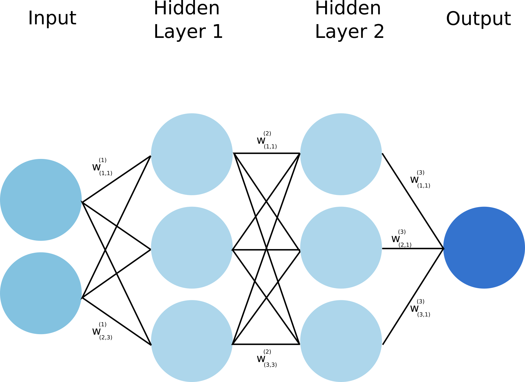
In the picture above, the input is transformed first through the hidden layer 1, then the second one and finally an output is predicted. Each transformation is controlled by a set of weights (and biases). During training, to indeed learn something, the network needs to adjust these weights to minimize the error (also called the loss function) between the expected outputs and the ones it maps from the given inputs. Using gradient descent [3] as an optimization algorithm, the weights are updated at each iteration as:

where L is the loss function and  is the learning rate.

As we can see above, the gradient of the loss with respect to the weight is substracted from the weight at each iteration. This is the so called gradient descent. The gradient  can be interpreted as a measure of the contribution of the weight to the loss. Therefore the larger is this gradient (in absolute value), the more the weight is updated during an iteration of gradient descent. 

The minimization of the loss function task ends up being related to the evaluation of the gradients described above. We will review 3 proposals to perform this evaluation:

• Analytical calculation of the gradients.
• Approximation of the gradients as being:  , where .
• Backpropagation or reverse mode autodiff.

Before going into the details of these proposals, we will first clearly define our problem and simplify it for the sake of the discussion.

Problem Definition

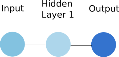
To simplify our discussion, we will consider that each layer of the network is made of a single unit, and that we have a single hidden layer. The network looks now like:

Let's discuss a little bit about how the input is transformed to produce the hidden layer representation. In neural network, a layer is obtained by performing two operations on the previous layer:

• First the previous layer is tranformed via a linear operation: the value of the previous layer is multiplied by a weight, and a bias is added to it. It gives: , where  is the value of the previous layer unit,  and  are respectively the weight and the bias discussed above.
• Second, the previous linear operation is used as an input to the activation function of the unit. This activation is generally chosen to introduce non linearity in order to solve complex tasks. Here we will simply consider that this activation function is a sigmoid function: . As a consequence the value y of a layer can be written as: .

So now, considering our case, with an input layer, one hidden layer, and an output layer, all made of a single unit and respectively called x, h and y, we can write:

, where  and  are respectively the weight and the bias used to compute the hidden unit from the input.

, where  and  are respectively the weight and the bias used to compute the output from the hidden unit.

From now on, we are able to calculate the output y based on the input x, through a set of transformations. This is the so called forward propagation since this calculation goes forward inside the network.

We now need to compare this predicted ouptut to the true one . As explained earlier, we use a loss function to quantify the error that the network does while prediciting. Here we will consider as a loss function the squared error defined as :

As discussed earlier, the weights (and biases) need to be updated according to the gradient of this loss function L with respect to these weights (and biases). Therefore the challenge here is to evaluate these gradients. The first approach would be to manually derive them.

Analytical differentiation

Although this method is cumbersome and error prone, it is worth to investigate to better understand the challenge Here we simplify a lot the problem since we have a single hidden layer and a single unit per layer. And yet the analytical derivation requires quite some attention.

Knowing that , we get :

Here we derived the gradient with respect to , and the calculation for the one with respect with  would be even more tedious. Therefore such an analytical approach would be very hard to implement for a complex network. In addition, computing wise this approach would be quite inefficient since we could not leverage the fact that the gradients share some common definition as we will soon discuss. A way more easy way to get these gradients would be to use a numerical approximation.

Numerical differentiation

Trading accuracy for simplicity, we can obtain the gradient using the following :

, with 

As suggested above, although simpler than the analytical derivation, this numerical differentiation is also less precise. In addition for every gradients to evaluate, we would have to calculate the loss function at least once (doing one forward pass by weights and biases). For a neural network with 1 million weigth parameters, it would requires 1 million forward passes, which is definitely not efficient to compute. Let's now come to a better solution and the core of this article by reviewing the backpropagation approach.

Backpropagation

Before speaking in more details about what backpropagation is, let's first introduce the computational graph that leads to the evaluation of the loss function.

The nodes in this graph correspond to all the values that are computed in order to get the loss L. If a variable is computed by applying an operation to another variable, an edge is drawn between the two variable nodes. Looking at this graph, and making use of the chain rule of calculus, we can express the gradient of L with respect to the weights (or biases) as:

Same goes for the weight :

One very important thing to notice here is that the evaluation of the gradient  can reuse some of the calculations perfomed during the evaluation of the gradient . It is even clearer if we evaluate the gradient :

We see that the first four terms on the righ hand of the equation are the same than the one from .

As you can see in the equations above, we calculate the gradient starting from the end of the computational graph, and proceed backward to get the gradient of the loss with respect to the weights (or the biases). This backward evaluation gives its name to the algoritm: backpropagation. The backpropagation algorithm can be illustrated by the image below:

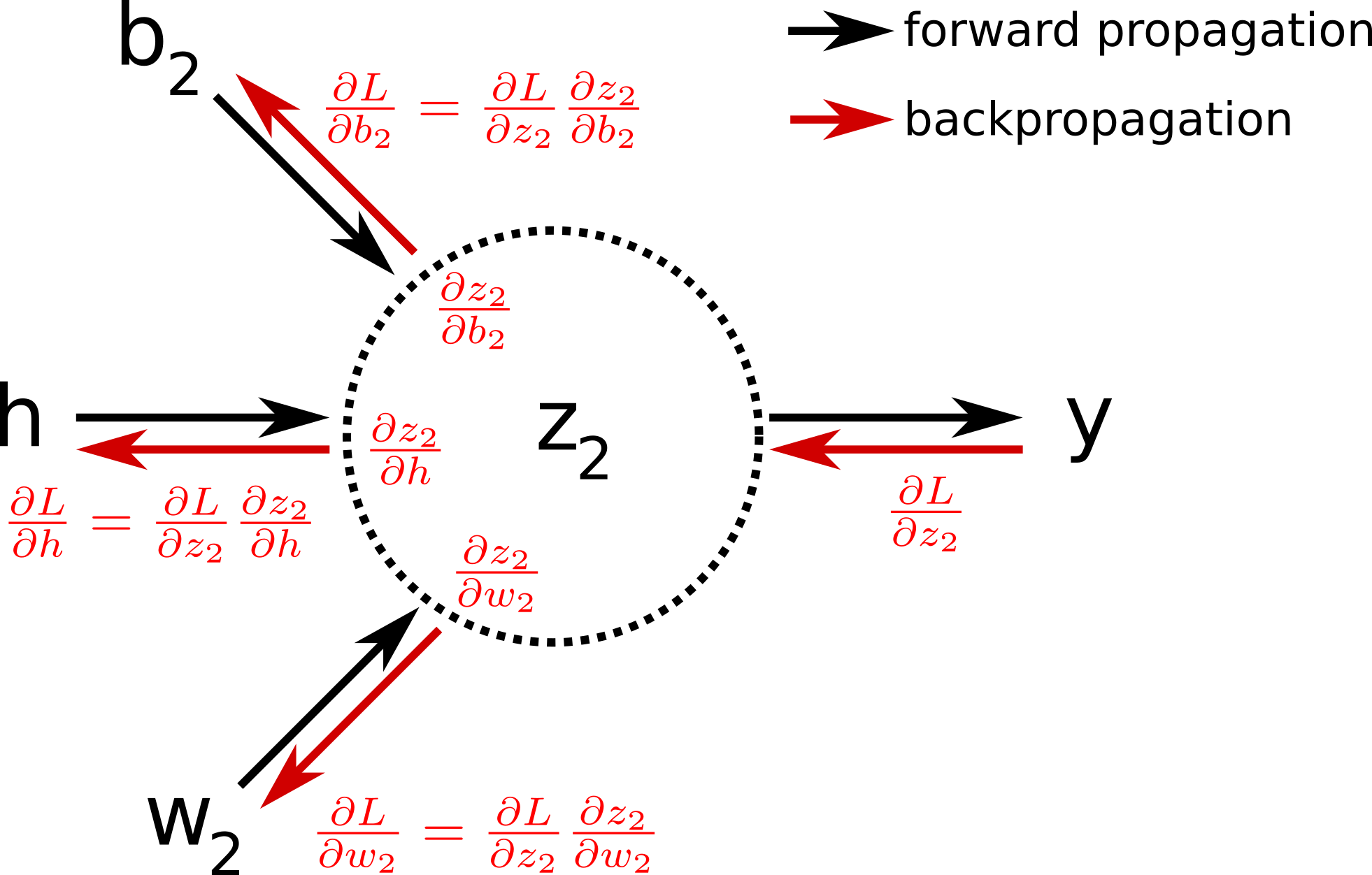
In pratice, one iteration of gradient descent would now require one forward pass, and only one pass in the reverse direction computing all the partial derivatives starting from the output node. It is therefore way more efficient than the previous approaches. In the original paper about backpropagation published in 1986 [4] , the authors (among which Geoffrey Hinton) used for the first time backpropagation to allow internal hidden units to learn features of the task domain. 

To visualize better what backpropagation is in practice, let's implement a neural network classification problem in bare numpy. Indeed as we will see below, there is no need of a complex deep learning library to play at first with a neural network.

A toy problem

Let's consider a binary classification problem where the task is about predict the class of a given input. All the code of this can be found in this Kaggle notebook [6].

The dataset

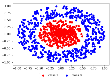
As a dataset, we chose a pretty standard not linearly separable dataset made of two classes "0" and "1". 

The neural network

As we can see from the dataset above, the data point are defined as . Therefore the input layer of the network must have two units. We want to classify the data points as being either class "1" or class "0", then the output layer of the network must contain a single unit. Between the input and the output layers, we add a hidden layer with 3 units. The full network looks like:

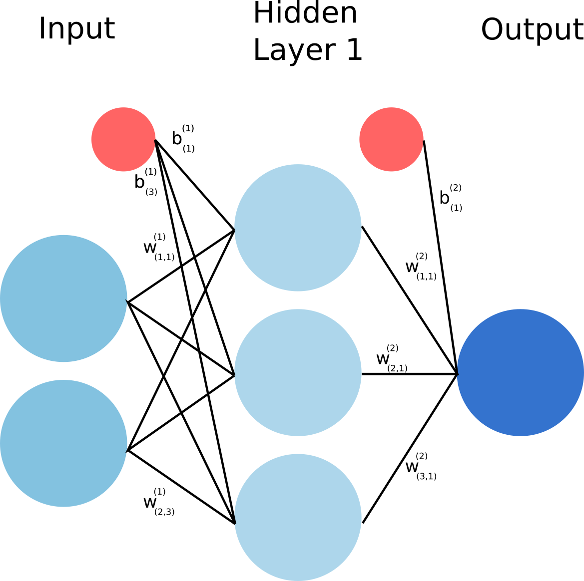
Choosing the right network architecture is more an art than a science, and there is no ground reason to choose the second layer to have 3 units. I encourage you to go and play with the tensorflow playground to realize that [5]. We have already studied a similar architecture before but with a single unit per layer. The previous equations can be easily generalized for layers with more than one unit:

 with , , and 

, with  and 

The above equations allow to predict a single output given a single data point . Instead of looping over all the data points from the dataset and evaluate y from them, it is way more efficient to take advantage of the vectorization of the problem. Let's consider the vector  with the shape :

where the upperscripts  simply refer to the datapoints.

We can rewrite the equations vectorized:

 with   a vector of shape  whose elements are all 1. 

Forward propagation

Let's now implement the code for the forward propagation through the network.

weights = {
    'W1': np.random.randn(3, 2),
    'b1': np.zeros(3),
    'W2': np.random.randn(3),
    'b2': 0,
}

def forward_propagation(X, weights):    
    # this implement the vectorized equations defined above.
    Z1 = np.dot(X, weights['W1'].T)  + weights['b1']
    H = sigmoid(Z1)
    Z2 = np.dot(H, weights['W2'].T) + weights['b2']
    Y = sigmoid(Z2)    
    return Y, Z2, H, Z1

Loss function

Previously, for simplicity we used the squared error as a loss function. It turns out that for a classification problem, this is not an appropriate choice as a loss function. Indeed the squared error is not able to distinguish bad prediction from extremely bad ones in a classification context. Here as a loss function, we will rather use the cross entropy function defined as:

where  is the output of the forward propagation of a single data point , and  the correct class of the data point.

To understand why the cross entropy is a good choice as a loss function, I highly recommend this video from Aurelien Geron [7].

Backpropagation

We have everything we need now to define the back_propagation function. First let's write again down the gradient equations:

We therefore need the following partial derivatives, which can be easily obtained:

We can now define the code for the backpropagation:

def back_propagation(X, Y_T, weights):
    N_points = X.shape[0]
    
    # forward propagation
    Y, Z2, H, Z1 = forward_propagation(X, weights)
    L = (1/N_points) * np.sum(-Y_T * np.log(Y) - (1 - Y_T) * np.log(1 - Y))
    # back propagation
    dLdY = 1/N_points * np.divide(Y - Y_T, np.multiply(Y, 1-Y))
    dLdZ2 = np.multiply(dLdY, (sigmoid(Z2)*(1-sigmoid(Z2))))
    dLdW2 = np.dot(H.T, dLdZ2)
    dLdb2 = np.dot(dLdZ2.T, np.ones(N_points))
    dLdH = np.dot(dLdZ2.reshape(N_points, 1), weights['W2'].reshape(1, 3))
    dLdZ1 = np.multiply(dLdH, np.multiply(sigmoid(Z1), (1-sigmoid(Z1))))
    dLdW1 = np.dot(dLdZ1.T, X)
    dLdb1 = np.dot(dLdZ1.T, np.ones(N_points))
    
    
    gradients = {
        'W1': dLdW1,
        'b1': dLdb1,
        'W2': dLdW2,
        'b2': dLdb2,
    }
    return gradients, L

Training: gradient descent

We have all in place to start training our network using gradient descent. Remember, at every iteration the weights and the biases are updated as.

epochs = 2000
epsilon = 1
initial_weights = copy.deepcopy(weights)

losses = []
for epoch in range(epochs):
    gradients, L = back_propagation(X, Y, weights)
    for weight_name in weights:
        weights[weight_name] -= epsilon * gradients[weight_name]
        
    losses.append(L)
    

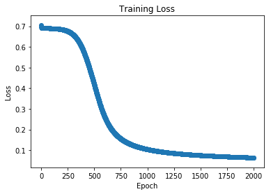
As we can see in the plot above where the loss is plotted with respect to the number of epochs the network experienced, we clearly observed a decrease of the loss. In other words, the network seems to make less and less errors. In other words, it learns something.

Visualize what the network learned

Using this visualization function, we can see how our network would classify a full map of points:

def visualization(weights, X_data, title, superposed_training=False):
    N_test_points = 1000
    xs = np.linspace(1.1*np.min(X_data), 1.1*np.max(X_data), N_test_points)
    datapoints = np.transpose([np.tile(xs, len(xs)), np.repeat(xs, len(xs))])
    Y_initial = forward_propagation(datapoints, weights)[0].reshape(N_test_points, N_test_points)
    X1, X2 = np.meshgrid(xs, xs)
    plt.pcolormesh(X1, X2, Y_initial)
    plt.colorbar(label='P(1)')
    if superposed_training:
        plt.scatter(X_data[:N_points//2, 0], X_data[:N_points//2, 1], color='red') 
        plt.scatter(X_data[N_points//2:, 0], X_data[N_points//2:, 1], color='blue') 
    plt.title(title)
    plt.show()

First let's plot how the network would classify the map before the learning process.

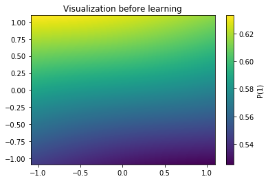
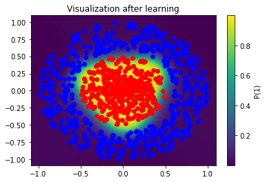
The picture above represents as a colormap the probability of a point being of class 1. As expected, the network is completely unable yet to classify correctly. Let's visualize the same thing after learning:

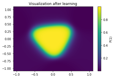
Now an island of class "1" lives in the middle of the map, while the rest is of class 0. If we superimpose the training samples to this visualization we realize that our network did a pretty good job classifying this map.

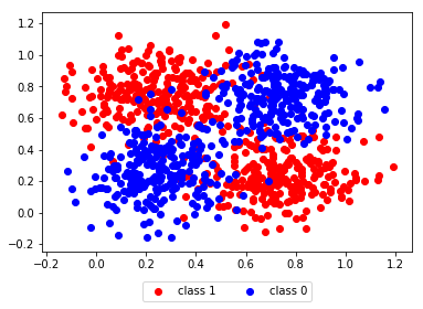
Bonus: Classify a XOR like distribution

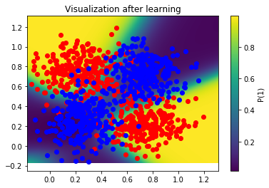
Considering the following XOR like distribution, we can use the same network architecture to classify it.

After learning, we plot as before the following map, and we observe that our network learns to classify reasonably well.

Conclusion

As a conclusion, backpropagation is not an extremely complicated algorithm, and as we have seen above, it is pretty straightforward to derive a bare numpy implementation for it. Although it comes out of the box with most of the deep learning frameworks, it is a good idea to get your hands dirty and understand a little bit more what it does. In some occasions, it might help you understand why your network is not learning properly.

[1] Train a convolutional neural network to classify cats and dogs

[2] "Yes, you should understand backprop", A. Karpathy

[3] Gradient descent, Wikipedia

[4] "Learning representations by back-propagating errors", D. Rumelhart, G. Hinton & R. Williams

[5] Tensorflow playground

[6] Kaggle notebook

[7] "A Short Introduction to Entropy, Cross-Entropy and KL-Divergence", A. Geron

Cover picture credit: Ivan Emelianov